exreport Fast, Reliable and Elegant Reproducible Research

Available examples:

Machine Learning Weka Example Basic

Introduction

In this example we make use of the wekaExperiment dataset that is packaged with exreport. This datasets represents a series of experiment in which several Machine Learning classifiers are compared by using a set of public datasets (UCI repository) as benchmark. The performance measures are the classification accuracy and the training time and have been obtained from a 10-fold cross-validation.

The wekaExperiment contains a variable for the method and dataset and two variables for the respective outputs. The datasets contains two parameters, the mentioned fold of the cross-validation for each entry and an additional boolean parameter to indicate if feature selection has been performed or not in the execution.

library(exreport)
colnames(wekaExperiment)

## [1] "method"           "dataset"          "featureSelection"
## [4] "fold"             "accuracy"         "trainingTime"

In this example we will start with a basic workflow in which we will compare the performace regarding accuracy of the different methods. For that we will follow the proposed scheme for an exreport procedure: "Process, Validate, Describe, Visualice"

We will start by loading the experiment into an exreport object, notice that we must indicate that the numeric variable "fold" is in fact a parameter.

experiment <- expCreate(wekaExperiment, name="weka", parameters=c("fold"))

A first look into the object shows us the different number of methods and datasets of our experiment as well as he different parameters and outputs. We can also access the raw data of the experiment by obtaining the coresponding parameter:

summary(experiment)

## 1) Experiment weka loaded from a data set.
##
## experiment
##
## #method: NaiveBayes, J48, RandomForest, OneR
## #dataset: hypothyroid, liver-disorders, vehicle, car, ionosphere, soybean, vote, anneal, lymph, vowel, audiology, glass, primary-tumor, balance-scale, horsecolic
##
##
## #parameters: featureSelection, fold
## #outputs: accuracy, trainingTime

# Print a few lines of random raw data
head(experiment$data)

##       method     dataset featureSelection fold accuracy trainingTime
## 1 NaiveBayes hypothyroid               no    0  94.9735       0.0824
## 2 NaiveBayes hypothyroid               no    1  93.6508       0.0177
## 3 NaiveBayes hypothyroid               no    2  93.6340       0.0065
## 4 NaiveBayes hypothyroid               no    3  94.9602       0.0059
## 5 NaiveBayes hypothyroid               no    4  95.2255       0.0045
## 6 NaiveBayes hypothyroid               no    5  95.7560       0.0045

Preprocessing

First of all, we will check the integrity of our experiment by checking that there are not repeated entries that would disrupt the analysis:

expGetDuplicated(experiment)

## experiment
##
## #method:
## #dataset:
##
##
## #parameters: featureSelection, fold
## #outputs: accuracy, trainingTime

The resulting experiment is empty, so we are allowed to continue

Before proceeding with any kind of analysis we must preprocess our results by performing the appropiate operations. We will begin by aggregating the result of the 10-fold cross validation performed for each method and dataset. For that, we reduce the fold parameter by using the mean function:

experiment <- expReduce(experiment, "fold", FUN = mean)
# Print a few lines of random raw data
head(experiment$data)

##         method   dataset featureSelection accuracy trainingTime
## 1          J48    anneal               no 98.77529      0.03192
## 2   NaiveBayes    anneal               no 86.52808      0.00989
## 3         OneR    anneal               no 83.63296      0.00804
## 4 RandomForest    anneal               no 99.10737      0.03578
## 5          J48 audiology               no 75.29644      0.01859
## 6   NaiveBayes audiology               no 68.65612      0.00545

Our first objetive will be to compare the different methods given its accuracy results, for that we first need to obtain a particular configuration of the parameters. Now that the fold parameter has been removed we have to deal with the featureSelection one. In our first test we want to compare the experiments performed when this parameter is set to "no", so we perform a subset operation.

experiment <- expSubset(experiment, list(featureSelection = "no"))

Now that we have a single configuration we instantiate the methods with the available paramaters. In this case, the featureSelection can be removed as it is unary:

experiment <- expInstantiate(experiment, removeUnary = T)

Evaluation

Our experiment is now ready to be validated by using statistical tests. In this case we have more than two methods, so we will choose a multiple comparison test. We want to obtain a ranking among the methods and decide which one is the best one, for that we will perform a "testMultipleControl" test, including a Friedman test followed by a post-hoc test using the Holm procedure. As the target variable is the accuracy, the test will measure maximization.

testAccuracy <- testMultipleControl(experiment, "accuracy", "max")
summary(testAccuracy)

## ---------------------------------------------------------------------
## Friedman test, objetive maximize output variable accuracy. Obtained p-value: 1.1365e-04
## Chi squared with 3 degrees of freedom statistic: 20.8400
## Test rejected: p-value: 1.1365e-04 < 0.0500
## ---------------------------------------------------------------------
## Control post hoc test for output accuracy
## Adjust method: Holm
##
## Control method: RandomForest
## p-values:
##             J48	0.5716
##      NaiveBayes	0.0324
##            OneR	0.0001
## ---------------------------------------------------------------------

The test show that there is a clearly hierarchy between the methods, and that some of them are statistically superior to the others. In the next section we will summarize this results and generate some graphics and tables.

Visualization

The previous test show that our results are promising, however we may want to observe at detail the results. For that exreport is packed with many plots and tables.

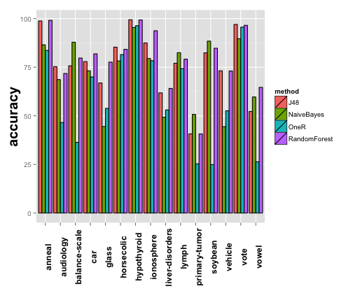
We will start by obtaining a visual overview of the performance of the methods. For that, we can summarize the experiment with an appropiate bar plot. There is a perfect built in function to achieve this:

plot1 <- plotExpSummary(experiment, "accuracy")
plot1

## [1] "Results for output \"accuracy\""

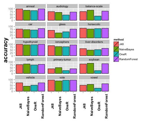
The plot is nice, but perhaps there are too much datasets and the results are not clearly displayed. Luckily, the majority of the graphical exreport functions can be parametrized, in this case, we will split the plot by methods.

plot1 <- plotExpSummary(experiment, "accuracy", columns = 3)
plot1

## [1] "Results for output \"accuracy\""

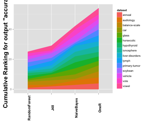
Next, we want to obtain additional information from the test we performed before. We will start by looking at the different ranks computed for the Friedman test, for that we have another built in function.

plot2 <- plotCumulativeRank(testAccuracy)
plot2

## [1] "Cumulative Ranking for Var accuracy"

The plot is a good representation of the results obtained by the test. However, we want to look at the results with some numeric precission. For that, we can generate a table using another built in function. In this case we generate a tabular summary for the test, in which we specify the different metric we need.

table1 <- tabularTestSummary(testAccuracy, columns =  c("pvalue", "rank", "wtl"))
table1

## $testMultiple
##                    method       pvalue     rank win tie loss
## RandomForest RandomForest           NA 1.666667  NA  NA   NA
## J48                   J48 0.5716076450 1.933333   9   0    6
## NaiveBayes     NaiveBayes 0.0324190828 2.800000  11   0    4
## OneR                 OneR 0.0001232936 3.600000  15   0    0

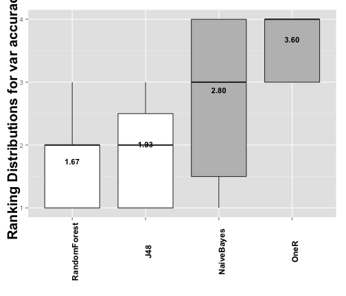
The final element we are going to create is a graphical representation of the Holm's post-hoc test using another built in functions, that generates a plot comparing the ranks distributions as well as the status of the test hypotheses.

plot3 <- plotRankDistribution(testAccuracy)
plot3

## [1] "Distribution of ranks for output \"accuracy\""

We are good with all of this new information, but surely we will be more confortable to study it out of the console, in fact, we need to discuss it with our coleages, so why not generating a nice graphical report?

Communicating

At this point we can collect all the output we have generated during this exreport workflow and pack it into a nice document. In this case we will be creating an interactive HTML report, from which we are going to b able to download the figures and the LaTeX code of the figures.

We start by initializing the report object:

report <- exreport("Your wekaExperiment example report")

And now it is time to add some content, be aware that the order of the elements in the report coincides with the order you add them. All the exreport objects have its own HTML and PDF representation, showing detailled summaries of their values and the operations performed with them.

# Add the experiment object for reference:
report <- exreportAdd(report, experiment)
# Now add the test:
report <- exreportAdd(report, testAccuracy)
# Finally you can add the different tables and plots.
report <- exreportAdd(report, list(plot1,plot2,table1,plot3))

At this point we would like to include an additional item in our report. We need a detailed table of our experiment, as we are preparing a scientific paper and we would like to have an overview of it to be included in an annex, despite the good summaries that we are providing with the plots and tests. Fortnunately, we have another built in function for this.

We have decided to generate the table at this point of the tutorial to discusse some special formating parameters of this function. Concretely, some of the tabular outputs generated by exreport have some properties that are only useful when rendering the objets in a graphic report, and have no effect in the object representation in the R console. In this case, we will tell the function to boldface the method that maximices the result for each column, and to split the table into to pieces when rendering.

# We create the table:
table2 <- tabularExpSummary(experiment, "accuracy", digits=4, format="f", boldfaceColumns="max", tableSplit=2)
# And add it to the report:
report <- exreportAdd(report, table2)

Now that we have finished adding elements to the report it is time to render it. We want to generate an HTML report, so we call the appropiate function, by default it renders and opens the report in your browser using a temporary file, but you can optionally specify a folder in which the report will be saved for future use.

# Render the report:
exreportRender(report, target = "HTML", visualize = T)